05. The 2D FFT
The 2D FFT
L2A45 2D FFT
2D FFT
Once the range bins are determined by running range FFT across all the chirps, a second FFT is implemented along the second dimension to determine the doppler frequency shift. As discussed, the doppler is estimated by processing the rate of change of phase across multiple chirps. Hence, the doppler FFT is implemented after all the chirps in the segment are sent and range FFTs are run on them.
The output of the first FFT gives the beat frequency, amplitude, and phase for each target. This phase varies as we move from one chirp to another (one bin to another on each row) due to the target’s small displacements. Once the second FFT is implemented it determines the rate of change of phase, which is nothing but the doppler frequency shift.
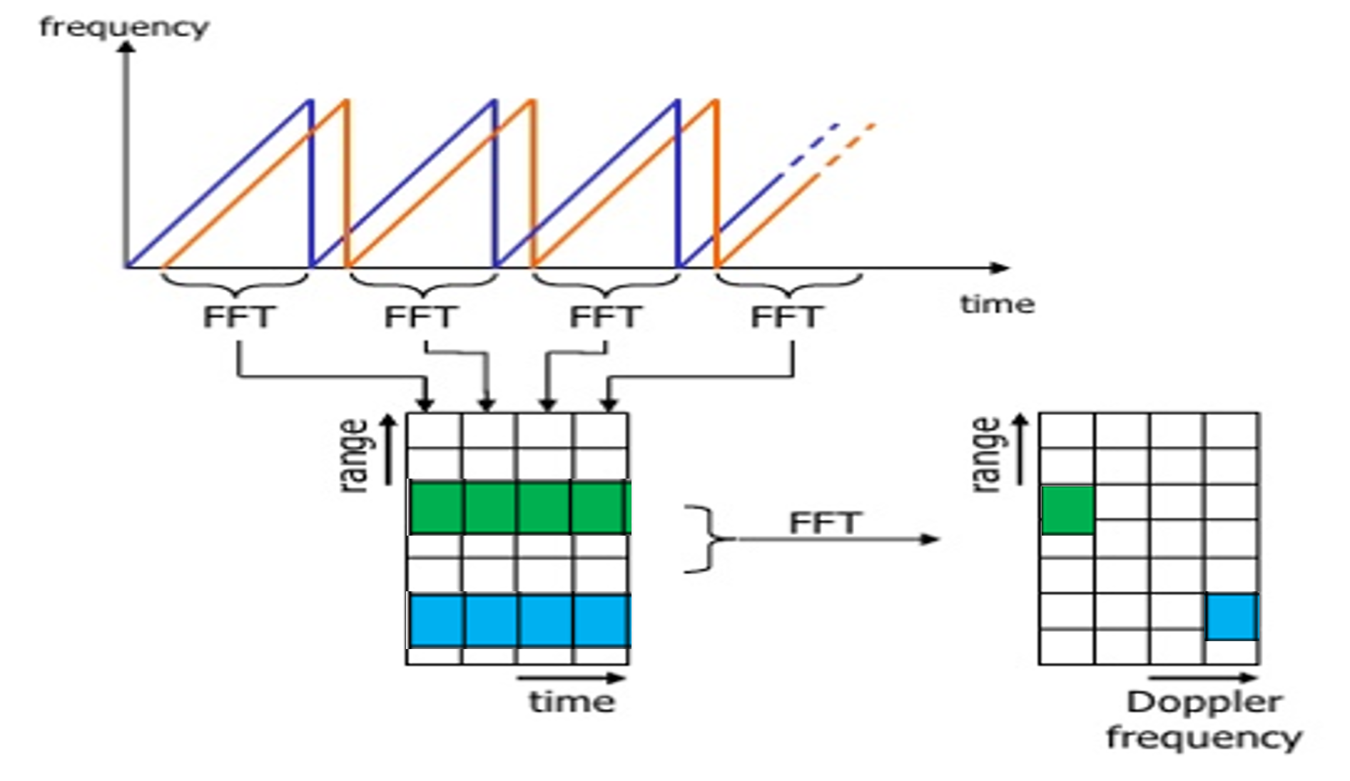
After running 2nd FFT across the rows of FFT block we get the doppler FFT. The complete implementation is called 2D FFT.
After 2D FFT each bin in every column of block represents increasing range value and each bin in the row corresponds to a velocity value.
The output of Range Doppler response represents an image with Range on one axis and Doppler on the other. This image is called as Range Doppler Map (RDM). These maps are often used as user interface to understand the perception of the targets.
2D FFT Output
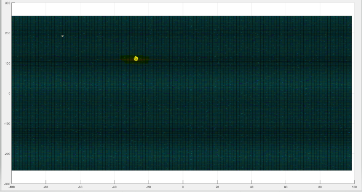
2D FFT output for single target. The x-axis here is the velocity and the y-axis is the range.
Range Doppler Map
source : rohde-schwarz
2D FFT Exercise
2D FFT In MATLAB
Steps to implement 2D FFT
The following steps can be used to compute a 2D FFT in MATLAB:
- Take a 2D signal matrix
- In the case of Radar signal processing. Convert the signal in MxN matrix, where M is the size of Range FFT samples and N is the size of Doppler FFT samples:
signal = reshape(signal, [M, N]);- Run the 2D FFT across both the dimensions.
signal_fft = fft2(signal, M, N);Note the following from the documentation :
Y = fft2(X)returns the 2D FFT of a matrix using a fast Fourier transform algorithm, which is equivalent to computingfft(fft(X).').'. IfXis a multidimensional array, then fft2 takes the 2-D transform of each dimension higher than 2. The outputYis the same size asX.Y = fft2(X,M,N)truncatesXor padsXwith trailing zeros to form an m-by-n matrix before computing the transform.Yis m-by-n. IfXis a multidimensional array, then fft2 shapes the first two dimensions ofXaccording to m and n.
- Shift zero-frequency terms to the center of the array
signal_fft = fftshift(signal_fft);- Take the absolute value
signal_fft = abs(signal_fft);-
Here since it is a 2D output, it can be plotted as an image. Hence, we use the
imagescfunction
imagesc(signal_fft);2D FFT Exercise
In the following exercise, you will practice the 2D FFT in MATLAB using some generated data. The data generated below will have the correct shape already, so you should just need to use steps 3-6 from above. You can use the following starter code:
% 2-D Transform
% The 2-D Fourier transform is useful for processing 2-D signals and other 2-D data such as images.
% Create and plot 2-D data with repeated blocks.

P = peaks(20);
X = repmat(P,[5 10]);
imagesc(X)

% TODO : Compute the 2-D Fourier transform of the data.
% Shift the zero-frequency component to the center of the output, and
% plot the resulting 100-by-200 matrix, which is the same size as X.
2D FFT Further Research